Johannes Rauh MPI MIS Inselstraße 22 04103 Leipzig jarauh@gmx.net
Seth Sullivant Department of Mathematics, NCSU Box 8205, Raleigh, NC 27695 smsulli2@ncsu.edu
June 19, 2014
This website explains how to obtain a Markov basis of the graphical model
of the complete bipartite graph K3,N with binary nodes. The computations
illustrate the theory developed in [6] that explains how to compute Markov
bases of toric fiber products.
We compute Markov bases of the binary (i.e. di = 2) hierarchical model of the complete
bipartite graph K3,N.
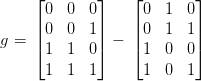
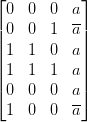
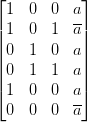
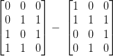
Theorem 1.For anyN, the Markov degree of the binary hierarchical model of thecomplete bipartite graph K3,Nis at most12.
The degree of the kernel Markov basis is at most 6, the degree of the PF Markov basisis 4 and the lifting defect is 2. Therefore, another bound on the degree of K3,Nis4+2N.
The proof of this theorem will take up Sections 2 to 5 of this manuscript. The proof will also
give an explicit description of a Markov basis of K3,N. In Section 6 we compare our theoretical
bounds with Markov bases that were obtained with 4ti2[1]. Both bounds are not sharp
for N ≤ 3.
The proof relies heavily on the lifting machinery developped in [6]. All the notation and all
the notions are explained in detail in that manuscript.
The idea of the proof is to use the fact that K3,N is a toric fiber product of N
copies of the three-star . The associated codimension zero product is a product of
copies of the graph 4 that arises from K4 by filling the triangle {1, 2, 3} filled (
). The calculation is complicated by the fact that the marginal cone of is not normal.
However, it turns out that all holes are vertices of the projected fibers. This allows to treat the
holes in a systematic way by adding additional inequalities to the inequality description of the
projected fibers. We compute the holes in Section 2.
The set of holes is described in Section 2. This allows to describe the projected fibers and to
calculate a PF Markov basis (Section 3). The liftings are computed in Section 4, where it is
also shown that the degree of the glued moves is at most 12. Section 5 presents a kernel
Markov basis of degree six. As it turns out, all moves from the kernel Markov basis are
redundant except for the quadratic moves. The appendix contains the kernel Markov basis
(Appendix A.1), the PF Markov basis (Appendix A.2) and the lifts (Appendix A.3) in tensor
notation.
The results in this manuscript were obtained with the help of Normaliz[2], 4ti2[1]
and Macaulay2[3]. This page contains links to files with code to reproduce the
results.
2. The holes of 4
In this section we study the set of holes of ℕ4. The following lemma summarizes the most
important properties:
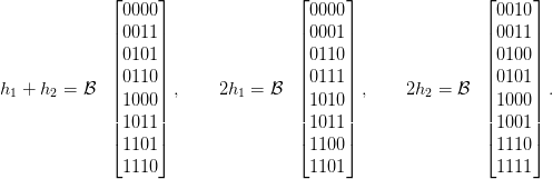
Lemma 2.The set of holes of ℕ4satisfies the following statements:
There are two fundamental holesh1,h2.
There is a partition 4 = 12of the rows of4such that the set of holes isgiven by (h1 + ℕ1)(h2 + ℕ2). The -margins of iare linearly independent fori = 1, 2.
There are linear functionals l1,l2 : ℤ4→ ℤ that satisfy the following: If a fiberF(b) has a holeh ∈ (hi + ℕi), then l3−i(v) > 0 = l3−i(h).
The lemma follows from the observations made in the remainder of this section. A
Macaulay2-program that does the calculations in this section can be found here.
A computation with Normaliz (input/output) shows that the Hilbert basis of the saturation
of ℕ4 contains two additional vectors h1,h2. Both restrict to the all-ones hole
h on the K4-marginals (that is, on all pair marginals). On the triangle-marginal,
h1 corresponds to XOR and h2 corresponds to the opposite of XOR. They are the
only fundamental holes, in the nomenclature of [4], as the following computations
show:
Consider one of the fundamental holes hi. According to [4], we need to do the
following:
Find the minimal non-negative solutions (λ,μ) of hi + λ = μ. This can be done,
for example, using 4ti2’s command zsolve.
(1 corresponds to XOR on the first three nodes, and 2 corresponds to its opposite). The
holes derived from h1 are of the form h1 + 1λ, where λ ∈ ℕ8. By symmetry, the holes derived
from h2 are h2 + 2μ, where μ ∈ ℕ8.
Consider the two linear forms
l1
= y000123 + y011123 + y101123 + y110123,
l2
= y001123 + y010123 + y100123 + y111123,
where yijk123 counts the coordinates where the (123)-marginal is equal to ijk (that is, l1
counts the XOR-part of the triangle-margin, and l2 counts the opposite XOR-part).
Then
Therefore, each hole is either derived from h1 or from h2, that is, (h1 + ℕ1) ∩ (h2 + ℕ2) = ∅.
Each set i is linearly independent. Hence different choices of the λ (or μ) give different
holes. Moreover, also the vectors -marginals of i are linearly independent for each i.
Therefore, no two holes of the same type have the same -marginals. Therefore, no projected
fiber contains more than one hole of the same type. A projected fiber can have one hole of each
type, though (for example, the holes h1 + 1(1,…, 1)t and h2 + 2(1,…, 1)t have the same pair
marginals and lie in the same fiber).
Let h = h1 + 1λ be a hole. If v belongs to the same projected fiber as h, then
v = 1λ′ + 2μ′ with λ′,μ′∈ ℕ8. As mentioned above, the -pair marginals of 1 are linearly
independent. Therefore, if μ′ = 0, then, since h and v have the same -marginals, h = v. Hence,
if v≠h is not a hole itself, μ′≠0. It follows that l2(m) > 0 = l2(h).
3. The projected fiber Markov basis
By Lemma 2, every hole is a vertex of its projected fiber, supported either by l1
or l2. Thus we can do the following: We start with an inequality description of the
semigroup ℕ4. This gives us a set of valid inequalities Du ≥ c for each projected
fiber. These inequalities are also valid for the holes. We augment the matrix D by
two additional rows corresponding to l1 and l2 and denote the augmented matrix
by D′. Then each projected fiber equals a solution set of linear inequalities of the form
D′u ≥ c′. Therefore, any inequality Markov basis of D′ can be used as a PF Markov
basis.
Each projected fiber is a subset of ℤ8, with basis e000,e001,…,e111. Let y000,…,y111 be the
corresponding coordinates. In a projected fiber, there are relations
y011
= y01− y000− y001− y010,
y101
= y02− y000− y001− y100,
y110
= y03− y000− y010− y100,
y111
= 1 − y01− y02− y03 + 2y000 + y001 + y010 + y100,
where yji is the sum of those marginals where the ith entry equals j. Since the projected fiber
is four-dimensional, these are all relations. An independent set of coordinates is given by
y000,y001,y010,y100 (that is, those coordinates with at most one one). According to
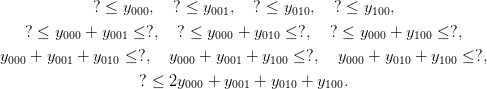
Normaliz (input/output), they satisfy inequalities of the form
To
get rid of the holes, we need to add the inequalities with linear parts l1,l2. In coordinates, they
take the form
The columns of the corresponding matrix D spans a lattice, and 4ti2 computes its Markov
basis (input/output). Since the first four rows of D form a unit matrix, D is easy to invert:
The first four coordinates of the Markov basis of D give the PF Markov basis in the
coordinates y000,y001,y010,y100. In tableau notation, PF Markov basis consists of the 16
moves, that are (up to symmetry; that is, up to a permutation of the columns) of the
form
−,
−,
−.
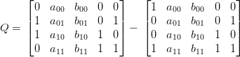
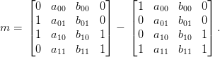
4. Lifting the PF Markov basis
In this section we compute the lifts. We use the algorithm described in [6] to compute
the lifting as an inequality Markov basis. Analyzing the results we find that the
maximal degree of a glue of lifts is bounded by 12. The file lift.m2 contains Macaulay2
code that does the calculations in this section. It makes use of further routines from
M2routines.m2.
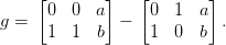
First consider
If b = a, then g lifts to
−,
− and −.
The lifting defect is at most two. Any move that arises by gluing lifts of g satisfies
Therefore, deg() ≤ 6.
If b =a, then g lifts to
−,
−, and −.
The lifting defect is at most two. Any move that arises by gluing lifts of g satisfies
Therefore, deg() ≤ 6.
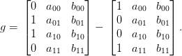
For
the lifts are (up to symmetry, exchanging the first two columns and state switching)
−, −
, −.
The lifting defect is at most two. Any move that arises by gluing lifts of g satisfies
Therefore, deg() ≤ 12.
For
the lifts are (up to symmetry, exchanging the first two columns and state switching)
−,
−,
−,
−
The lifting defect is at most two. Any move that arises by gluing lifts of g satisfies
Therefore, deg() ≤ 12.
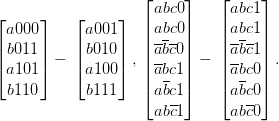
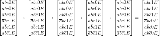
5. The kernel Markov basis in tableau notation
The Markov basis of computed by 4ti2 has 20 elements of degrees four and six (input/output).
In tableau notation, it consists of the following moves (up to symmetry, involving permuting
the first three columns):
Recall that the kernel Markov basis consists of quadratic moves of the form
and lifts that can be constructed from the moves in the Markov basis of by adding constant
columns in the tableau notation. The lifted moves have degree 4 and 6, and so the kernel
Markov basis has degree 6.
Let us show that all lifted moves from the kernel Markov basis are redundant; that is: We
only need the quadratic moves from the kernel Markov basis. In fact, consider, for example, a
lift m of degree six. The glues of lifts of the PF Markov basis contain the quadratic moves of
the form
and so on. Applying such quadratic moves reduces m to zero:
The quartic moves of the kernel Markov basis can be reduced similarly.
6. Comparison with computational results
For N ≤ 3, the Markov basis of K3,N can be computed (within reasonable time) using 4ti2.
The Markov degrees are:
N
1
2
3
deg
2
4
6
These three computed degrees are much smaller than the theoretical bound of min{4 + 2N, 12}.
K3,1 is a tree; hence the Markov degree is two. The additional moves obtained by lifting the
PF Markov basis are not necessary. For a zero-fold toric fiber product it is no wonder that our
bound is far from being tight.
A Markov basis of K3,2 was computed in [5] by interpreting K3,2 as a TFP of three
two-stars. Here, we interprete these moves from the viewpoint of our above computations. The
Markov basis of [5] consists of two kinds of quadrics and quartics. First, there are the
codimension-zero quadrics. Second, the quadrics of the two three-stars glue together and yield
further quadrics. Observe that the two interpretations of K3,2 interchange the roles of the
codimension-zero quadrics and the glued quadrics: The codimension-zero quadrics of
K1,2×′K1,2×′K1,2 correspond to the glued quadrics of K3,1×K3,1, and vice
versa.
The quartics are of the form
for some lij,mij∈{0, 1}, modulo a permutation of the first three rows. All of these quadrics are
glues of, say, m and m′. If either (a00,b00) = (a01,b01) or (a10,b10) = (a11,b11), then m is a
quadric; that is
Otherwise, m is the quartic
That is, m is a lift of
A g of this form may be quadratic or quartic, depending on the (aij,bij). One can see that
projecting the Markov basis of K3,2 gives the full PF Markov basis. Therefore, the reason that
the bound is not sharp is not that the PF Markov basis is too large, but that not all glues are
necessary.
A. Intermediate results in tensor notation
In this appendix we present some of the above results in tensor notation. These results are
straightforward translations of the output of 4ti2, without factoring out any symmetry or
other structures, and so they should be considered as intermediate steps on the way from the
raw 4ti2-output towards the form summarized above.
The tensor notation is as follows: Any state x ∈{0, 1}4 corresponds to a binary
string x0x1x2x3, which can be considered as the binary representation of a natural number.
The three least-significant bits correspond to the first group of nodes in K3,N. Identifying the
first 16 bitstrings with the letters from a to p, the states appear at the following
positions:
A.1. The kernel Markov basis in tensor notation
The Markov basis of computed by 4ti2 has 20 elements of degrees four and six:
+0
−0
−0
+0
−0
+0
+0
−0
,
0+
0−
0−
0+
0−
0+
0+
0−
,
+−
00
−+
00
−+
00
+−
00
,
00
+−
00
−+
00
−+
00
+−
,
+−
−+
00
00
−+
+−
00
00
,
00
00
+−
−+
00
00
−+
+−
,
+0
−0
0−
0+
−0
+0
0+
0−
,
0+
0−
−0
+0
0−
0+
+0
−0
,
+−
00
00
−+
−+
00
00
+−
,
00
+−
−+
00
00
−+
+−
00
,
+0
0−
−0
0+
−0
0+
+0
0−
,
0+
−0
0−
+0
0−
+0
0+
−0
,
2−
−0
−0
0+
2+
+0
+0
0−
,
+2
0+
0+
−0
−2
0−
0−
+0
,
+0
2 +
0−
+0
−0
2−
0+
−0
,
0+
+2
−0
0+
0−
−2
+0
0−
,
+0
0−
2+
+0
−0
0+
2−
−0
,
0+
−0
+2
0+
0−
+0
−2
0−
,
0+
−0
−0
2−
0−
+0
+0
2 +
,
+0
0−
0−
−2
−0
0+
0+
+2
.
A.2. The projected fiber Markov basis in tensor notation
The PF Markov basis consists of the 16 2 × 2 × 2-tableaus
+−
00
−+
00
,
00
+−
00
− +
,
+0
−0
−0
+0
,
0+
0−
0−
0 +
,
+−
−+
00
00
,
00
00
+−
− +
,
+0
0−
−0
0 +
,
0+
−0
0−
+0
,
+−
00
00
− +
,
00
−+
+−
00
,
+0
−0
0−
0 +
,
0−
0+
+0
−0
,
+−
+−
−+
− +
,
+−
−+
+−
− +
,
++
−−
−−
+ +
,
+−
−+
−+
+ −
.
A.3. Lifting in tensor notation
This Section contains the lifts in the raw form, as found by 4ti2.
For
there are ten lifts:
+−
−+
00
00
00
00
00
00
,
00
00
00
00
+−
−+
00
00
,
+−
00
00
−+
00
−+
00
+−
,
+−
00
−+
00
00
−+
+−
00
,
00
+−
−+
00
−+
00
+−
00
,
00
+−
00
−+
−+
00
00
+−
,
0+
0−
−0
+0
−0
+0
+0
−0
,
+0
−0
−0
+0
0−
0+
+0
−0
,
0+
0−
0−
0+
−0
+0
0+
0−
,
+0
−0
0−
0+
0−
0+
0+
0−
.
For
there are six lifts:
+0
−0
0−
0+
00
00
00
00
,
00
00
00
00
+0
−0
0−
0+
,
00
00
+−
−+
+0
−0
−0
+0
,
0+
0−
0−
0+
+−
−+
00
00
,
+−
−+
00
00
0+
0−
0−
0+
,
+0
−0
−0
+0
00
00
+−
−+
.
For
there are 21 lifts:
0+
0−
−0
+0
−0
+0
0+
0−
,
+−
−+
+−
−+
00
00
00
00
,
00
00
00
00
+−
−+
+−
−+
,
+−
−+
00
00
00
00
+−
−+
,
00
00
+−
−+
+−
−+
00
00
,
22
−+
00
−+
−+
00
+−
00
,
+−
2 2
+−
00
00
+−
00
−+
,
2−
2 +
0−
0+
−0
+0
+0
−0
,
+2
−2
+0
−0
0+
0−
0−
0+
,
00
+−
22
+−
−+
00
+−
00
,
+−
00
+−
2 2
00
−+
00
+−
,
0+
0−
2+
2−
−0
+0
+0
−0
,
+0
−0
+2
−2
0−
0+
0+
0−
,
+−
00
−+
00
22
+−
00
+−
,
00
+−
00
−+
+−
2 2
+−
00
,
+0
−0
−0
+0
2+
2−
0+
0−
,
0+
0−
0−
0+
+2
−2
+0
−0
,
+−
00
−+
00
00
−+
22
−+
,
00
+−
00
−+
−+
00
−+
22
,
+0
−0
−0
+0
0−
0+
2−
2 +
,
0+
0−
0−
0+
−0
+0
−2
+2
.
For
there are 40 lifts:
+−
−+
−+
+−
00
00
00
00
,
00
00
00
00
+−
−+
−+
+−
,
+−
−+
00
00
00
00
−+
+−
,
00
00
+−
−+
−+
+−
00
00
,
+−
00
−+
00
00
−+
00
+−
,
00
+−
00
−+
−+
00
+−
00
,
+0
−0
−0
+0
0−
0+
0+
0−
,
0+
0−
0−
0+
−0
+0
+0
−0
,
22
−+
−+
00
−+
00
00
+−
,
+−
2 2
00
+−
00
+−
−+
00
,
2−
2 +
−0
+0
−0
+0
0+
0−
,
+2
−2
0+
0−
0+
0−
−0
+0
,
+−
00
22
+−
00
−+
+−
00
,
00
+−
+−
2 2
−+
00
00
+−
,
+0
−0
2+
2−
0−
0+
+0
−0
,
0+
0−
+2
−2
−0
+0
0+
0−
,
+−
00
00
−+
22
+−
+−
00
,
00
+−
−+
00
+−
2 2
00
+−
,
+0
−0
0−
0+
2+
2−
+0
−0
,
0+
0−
−0
+0
+2
−2
0+
0−
,
00
+−
−+
00
−+
00
22
−+
,
+−
00
00
−+
00
−+
−+
22
,
0+
0−
−0
+0
−0
+0
2−
2 +
,
+0
−0
0−
0+
0−
0+
−2
+2
,
2−
−0
2+
+0
−0
0+
+0
0−
,
+2
0+
−2
0−
0+
−0
0−
+0
,
+0
2 +
−0
2−
0−
+0
0+
−0
,
0+
+2
0−
−2
−0
0+
+0
0−
,
+0
0−
−0
0+
2+
+0
2−
−0
,
0+
−0
0−
+0
+2
0+
−2
0−
,
0+
−0
0−
+0
−0
2−
+0
2 +
,
+0
0−
−0
0+
0−
−2
0+
+2
,
2−
−0
−0
0+
−0
0+
0+
+2
,
+2
0+
0+
−0
0+
−0
−0
2−
,
0+
+2
−0
0+
−0
0+
2−
−0
,
+0
2 +
0−
+0
0−
+0
−2
0−
,
+0
0−
2+
+0
0−
−2
+0
0−
,
0+
−0
+2
0+
−0
2−
0+
−0
,
0+
−0
−0
2−
+2
0+
0+
−0
,
+0
0−
0−
−2
2+
+0
+0
0−
,
References
[1]4ti2 team, “4ti2—a software package for algebraic, geometric and combinatorial
problems on linear spaces,” available at http://www.4ti2.de.
[2]W. Bruns, B. Ichim, and C. Söger, “Normaliz. Algorithms for rational cones and
affine monoids.” available from http://www.math.uos.de/normaliz.
[3]D. Grayson and M. Stillman, “Macaulay2, a software system for research in
algebraic geometry,” available at http://www.math.uiuc.edu/Macaulay2.
[4]R. Hemmecke, A. Takemura, and R. Yoshida, “Computing holes in semi-groups
and its applications to transportation problems,” Contributions to DiscreteMathematics, vol. 4, no. 1, 2009.
[5]T. Kahle, J. Rauh, and S. Sullivant, “Positive margins and primary
decomposition,” Journal of Commutative Algebra, 2014, accepted.
[6]J. Rauh and S. Sullivant, “Lifting markov bases and higher codimension toric
fiber products,” arXiv, 2014. [Online]. Available: http://arxiv.org/abs/1404.6392


 (
(


 and
and 

 that arises by gluing lifts of
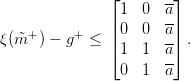
 )
) 


 that arises by gluing lifts of
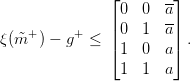
 )
) 


 that arises by gluing lifts of
 )
) 


 that arises by gluing lifts of
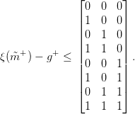
 )
) 
![[abcD E ] [abcD E ′]
′ ′ − ′
abcD E abcD E](K3N63x.png)
![[ ] [ ]
a b c d E a′b c d E
a′b′c′d′E − a b′c′d′E ,](K3N64x.png)
 ′
′